August, 2026
Extracting Surfaces from Gaussian Splats
This article was based on my work on next best view planning for 3D Gaussian splats. It explains how Poisson surface reconstruction (PSR) can be used to reconstruct the surfaces of a scene from 3D Gaussain splats (3DGS). First we will give background on PSR and 3DGS then we will discuss how to use to use Gaussian splats as input to PSR. Finally, we will briefly explain using stochastic surface reconstruction for next best view planning.
Background: Poisson Surface Reconstruction
Define the model as
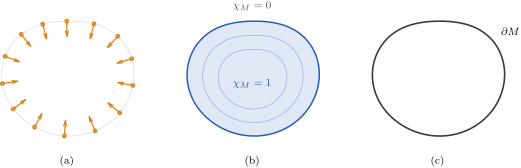
(a) the samples, each with an inward normal. (b) the indicator function reconstructed from them. (c) the surface, a level set of the indicator function.
The gradient of
so a set of normals sampled over
The input to the algorithm is
Expectation for Samples
- Each sample has a normal.
- Normals are consistently oriented. The sign of
- Samples lie on the surface. Zero mean noise in
- Sample density follows surface area. The weight
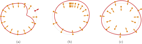
Grey is the true surface and red is the reconstruction. (a) one normal is flipped. (b) samples are concentrated on one arc and
Background: 3D Gaussian Splatting
3DGS represents a scene as a collection of Gaussians, each parameterised by a position, rotation, scale, opacity and a set of spherical harmonic coefficients. A view is synthesised by projecting the Gaussians into screen space and alpha blending them in depth order. The parameters are optimised by gradient descent against a photometric loss between the synthesised and source views. An adaptive density control algorithm periodically adds Gaussians in poorly represented regions of the scene and removes them from dense or transparent ones.
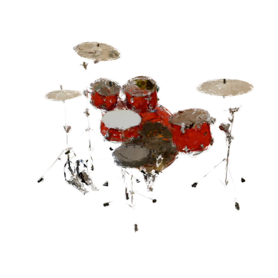
A synthetic drum scene reconstructed by 3DGS. The silhouettes are correct and the surfaces are not.
Sampling Normals from Gaussians
The direct approach treats each Gaussian as one sample. The position
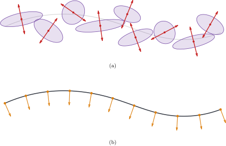
(a) a cross section of the Gaussians near a surface, with the axis of least variance of each drawn in red. (b) the sample normals which the surface requires.
This fails each of the four requirements.
- A Gaussian close to spherical has no well defined axis of least variance, and the photometric loss does not penalise one.
- The axis of least variance is an axis rather than a direction, so the sign of
- The Gaussians are not surface aligned. They overlap and extend to either side of the surface, so their positions are biased off it. Alpha blending hides this during rendering, because a set of overlapping Gaussians and a surface can integrate to the same image.
Sampling Normals in Image Space
Each of these problems is a consequence of reading geometry from individual Gaussians. Sampling the rendered images instead avoids them, because alpha blending combines the overlapping Gaussians before the sample is taken.

The pipeline. The stages between the input views and the point cloud produce a sample set which meets the requirements of the solve.
Surface Aligned Gaussians
Gaussian Surfels constrains each Gaussian to be flat by driving the third component of its scale to zero. A flat Gaussian has a well defined normal, which satisfies the first requirement. We use Gaussian Surfels with its additional regularisation terms removed, which simplifies comparison against the unmodified algorithm at the cost of some surface alignment.
Reconstructing Normals from Depth
The scene is rendered at each input pose
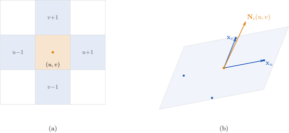
(a) the pixel and the four neighbours the central differences are taken across. (b) the same five pixels back projected into view space. The normal is perpendicular to both tangents.
A pixel is only shaded by a surface facing the camera which rendered it, so
Masking and Downsampling
The position and normal maps are downsampled with a
This holds only for blocks which are covered by the surface throughout. A block which straddles a silhouette back projects partly onto the surface and partly onto the background, and its average position lies off the surface. We accumulate a mask
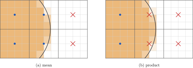
Downsampling across a silhouette. A blue dot marks a block which is kept and a red cross one which is rejected. (a) the mean keeps blocks which are mostly background. (b) the product keeps only blocks which are covered throughout.
The samples which pass the mask are transformed into world space by
Surface Uncertainty
For online capture of a scene it is useful to know where in the scene has not been appropriately covered. We can use the total uncertainty of a camera angle as a measure of it's importance.
Stochastic Poisson surface reconstruction (Sellán and Jacobson, reformulated by Holden et al.) reformulates PSR. The output is a Gaussian process over
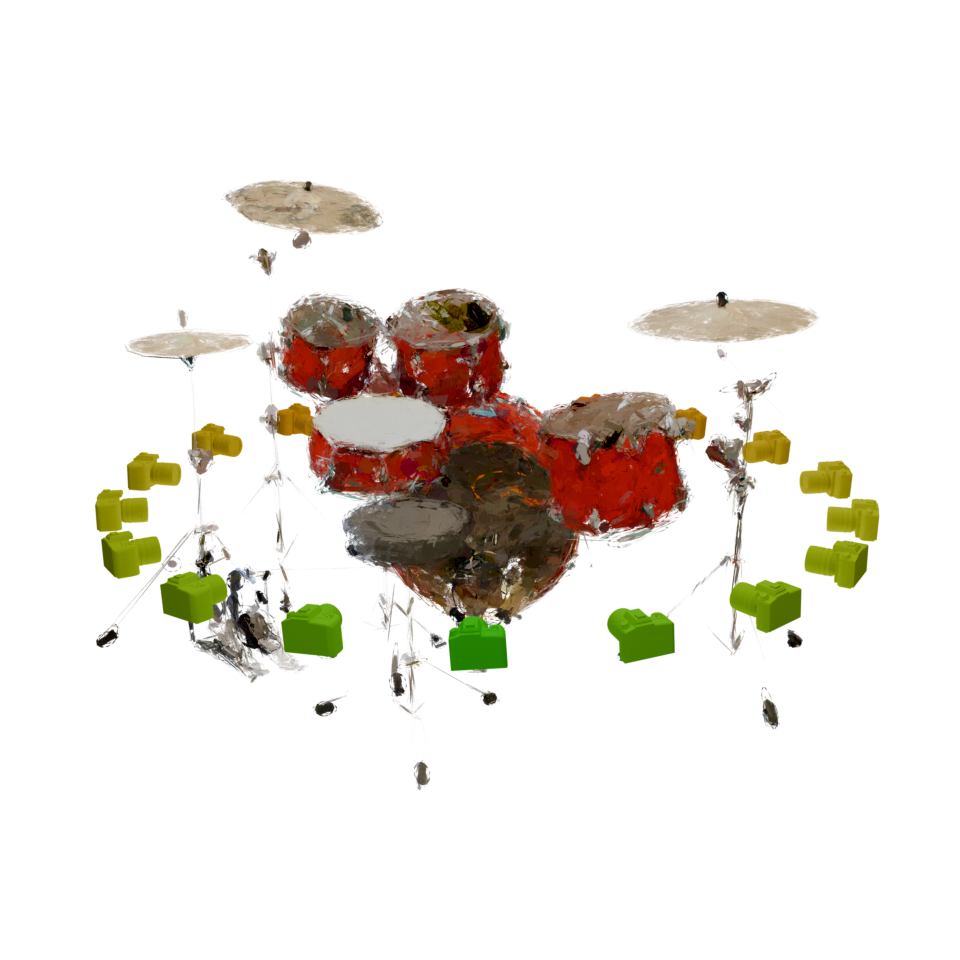
Candidate poses on the drum scene coloured by the surface uncertainty each captures, with green being more certain. The back of the kit was not covered by the input views.
Further Reading
- Kazhdan, Bolitho and Hoppe, Poisson Surface Reconstruction.
- Kerbl et al., 3D Gaussian Splatting for Real-Time Radiance Field Rendering.
- Dai et al., High-quality Surface Reconstruction using Gaussian Surfels.
- Sellán and Jacobson, Stochastic Poisson Surface Reconstruction.