August, 2026
Designing a Database for Non Volatile Memory

This article was inspired by AMD's dependency analysis for LLM decode. It assumes familiarity with databases and systems programming. It discusses how NVMe queue depth interacts with database design decisions.
Processors have been getting faster for decades. Unfortunately the time to read and write a file has not kept up. A modern non-volatile memory (NVM) drive answers a single 4 KiB random read in tens of microseconds, a thousand times slower than loading the same data from volatile memory.
Non-volatile memory includes devices such as solid state drives (SSD), M.2 cards and hard disk drives.
Databases are asked to hide this gap. We are going to design one that responds to requests quickly (low latency) and handles many requests at once (high throughput) using a simplified model of NVM drives. We discuss why to shard per core, how to choose a storage format, and how to pipeline requests. We finish with a brief discussion of a request's latency distribution.
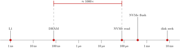
Approximate service times, log scale.
The Database API
For the purposes of this article we are going to assume Cassandra's CQL interface. It looks like SQL but is more restrictive, specifically:
- Rows are divided into partitions, identified by a partition key (a partition contains multiple rows).
- Rows within a partition are stored in order of the clustering key.
- Normal reads and writes name a single partition key.
- There are no joins or foreign keys (schemas are denormalised).
- Secondary indexes are declared explicitly.
CQL is designed this way so requests can be handled by a single shard. Sharding divides a table's rows into groups, and different shards may be stored on distinct drives or machines. Partition keys let us route a request directly to the shard holding the relevant partition. Some requests do need data from several partitions, and potentially several shards. In this case the request is scattered among the shards and then gathered to form a final answer. Cassandra's data modelling guide may be useful for understanding the implications of Cassandra's design.
Constraining our database's interface allows the following analysis to be more specific, although the same factors apply to most databases.
Model of NVM Drive
An NVM drive is best utilised when it holds many read or write operations at once. A drive contains many independent flash dies. Software which waits for a response before making another operation leaves most of these dies idle. The drive has a queue of operations submitted but not completed.
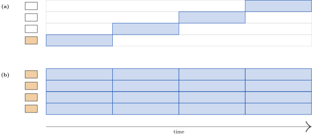
Rows are dies within the NVM drive. The orange boxes on the left are number of operations in the queue. (a) Submit a single operation and wait for the response before submitting another. (b) Submit four operations at once.
Let the average size of the queue be
The drive also has a ceiling for how well it can parallelize. However many operations we offer, it retires at most
Throughput
The two bounds cross at a queue depth called the saturation point.
Below
The heavily simplified model is based on The Operational Analysis of Queueing Network Models.
Example: Micron 7450 PRO
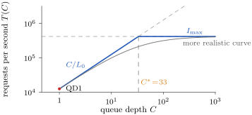
Throughput for a Micron 7450 PRO under a 70/30 mix. QD1 is the operations per second at queue depth one. The grey curve is an approximation of the real drive.
The Micron 7450 PRO is an enterprise NVMe drive. Its 7.68 TB E1.S model answers a 4 KiB random read in
We expect to be able to issue 33 operations at once before operations start to take longer. The below table illustrates these diminishing returns.
Database design
One shard per core
Our model tells us that we should maximize the queue depth enough to reach the point of diminishing returns. The most straightforward way is multithreading. We divide partition ownership among threads and use the partition key to route each query. To avoid contention we have each thread own it's caches and files. If we have enough connections making requests touching different shards we can may be able to saturate the drive using this technique alone.
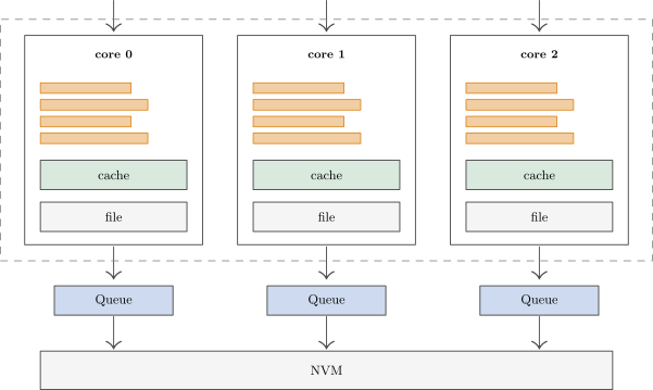
One shard per core, each owning a disjoint set of partitions. A request is routed by hashing its partition key. A request naming several partitions is split across several shards.
We can also pin each shard to a core, which tells the operating system not to move the thread to another core. Pinning has the trade-off that a busy shard cannot use an idle core's capacity. This may cause a lower average throughput but allows more consistent latency, we will return to this trade-off when discussing tail latency.
Since I/O operations are much slower than compute we don't want our threads to wait for a response. We could have a thread per request but this requires more work and memory from the OS. We instead make each request's handler into a coroutine: a function that can suspend part-way through, return control to the thread, and resume later from where it stopped. A request suspends it's coroutine when it submits an I/O operation and resumes when the answer arrives. Unfortunately, since we are touching the same shard's shared resources we can't simply overlap the I/O for different request coroutines, this is where pipelining will come in.
B-trees or LSM
The format we store our table's rows deeply effects which I/O operations we make. We will consider two choice, B-Trees or log structured merge (LSM) trees. A B-tree keeps rows in one sorted structure and updates it in place. Its pages form a shallow tree in which each page holds keys and the locations of the pages below it. A log-structured merge tree instead keeps several sorted runs of pages, newest first, and merges them in the background (compaction). The two structures differ in how they utilize I/O.
- When searching a B-tree, a parent node's page must be read before we know which child page to read.
- When searching an LSM tree we can load multiple pages at once but we need to issue more reads in total.
- Modifying a B-tree requires more writes up-front but compaction of an LSM tree requires more writes in total.
Under this analysis the LSM tree allows more drive queue depth (
Requests Lifecycle
We break read and write requests into smaller components and map the dependencies between them. This will allows us to overlap and combine operations from different queries. The analysis focuses on I/O, which dominates compute cost. Costs are approximated relative to one uncached drive read (
| Tag | Stage | I/O | Cost |
|---|---|---|---|
nw | read the request frame from the socket | usually one receive | 1 to 3 |
pti | descend one level of the partition or clustering tree | one read | 1 or cached |
rw | read the row/s the leaf points at | usually one read | ~1 (batched) |
ixi | descend one level of one secondary index | one read | 1 or cached |
wa | append the whole transaction to the log | one sequential write, sized by the pages dirtied | ~1 (batched) |
fl | flush the log to durable media | one barrier | ~35 or ~0 with power-loss protection |
rs | write the response frame | usually one send | 1 to 3 |
ck | write the dirtied pages back to the data file | one write per page, deferred | ~1 per page |
Write
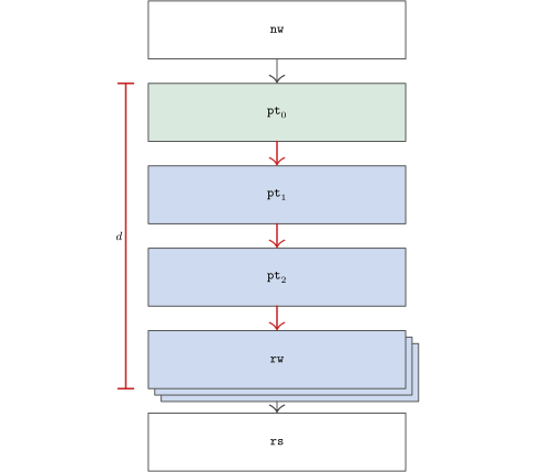
A read of one row. Every stage waits on the one above it, so
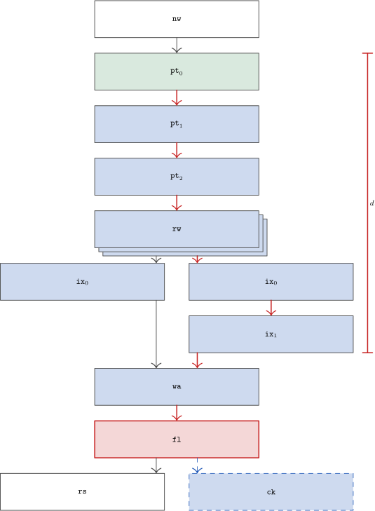
A write against a table with a clustering key and two secondary indexes, one of them a level deeper than the other. The longest chain runs through the deeper index, giving
The steps have the following relationships:
nwandrsare independent per connection.pti is irreducible. A page must be read before we know which page follows it.rwcan be batched and parallelized. Adjacent rows and overflow pages are laid out in order, so they can be issued together.ixi requiresrw. Removing the stale index entry requires the old column value.ixi needs a global lock. An index has a global lock which covers every partition, so two requests on different partitions contend for the index.wacan be submitted in parallel with the transactionckmust followfl. If a page reached the data file before the log covering it was durable, a crash between the two would leave a partially updated file and no record with which to repair it.ckis otherwise unconstrained. Once the log is durable the pages may be written at any time.
Pipelining Between Requests
Two read requests naming different partitions can naturally interleave without coordination. We ensure that a thread does not lock on read and ensure that our clients take advantage by opening multiple connections. Unfortunately we can't pipeline write requests to ensure our tree remains in a consistent state. This means stalling on writes.
We can also trivially pipeline the network calls. The write ahead log can also be pipelined but since we still need to commit before returning to ensure durability. we instead batch with a limit on the number of batched requests.
Tail latency
It was mentioned earlier that sometimes we may trade lower average latency for consistency (low variance).
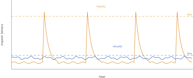
Two database engines with different latency distributions. The bursty engine has a lower mean latency but a much higher
We reduced variance by:
- Pinning shards to cores.
- Choosing B-trees as our storage format.
On the other hand we increased variance by:
- Batching flushes across requests
There is a trade-off between variance and mean, similar to the trade-off between memory and compute. Our database design allows us to tune this trade-off by, for example, changing the flush batch size.
The database design we justified is plexdb, an experimental database which supports the CQL interface. It is shard-per-core and coroutine-driven, stores rows in B-trees, and pipelines and batches I/O.
Further reading
- An In-Depth Overview of NVMe and NVMe-oF
- Lazowska, Zahorjan, Graham and Sevcik, Quantitative System Performance. Chapter 5 derives the asymptotic bounds and the saturation point used above.
- Denning and Buzen, The Operational Analysis of Queueing Network Models. The paper the bounds come from.