September, 2023
Image Segmentation of Kidney Microscope Slides
The HuBMAP Kidney Segmentation challenge on Kaggle challenges an AI to segment regions of microvascular (blood vessels) from other tissue in a microscope slide of a healthy human kidney. Each pixel from a stained slide of the kidneys should be labeled as part of a vein or not. This page explores using a deep convolutional neural network to sole this problem. Otsu's segmentation is used as an example of a simpler, but ineffective approach, which justifies the machine learning approach.
Slide and Label Data
Whole Slide Images (WSIs) from periodic acid-Schiff stained tissues slides were obtained from five healthy adults. These slides were split into blood_vessel, glomerulus, and unsure. The labels are given per tile as a list polygons for each label. The model should predict a blood_vessel label for an unlabelled tile.
Background
Semantic segmentation is the task of clustering parts of images together which belong to the same object class.
There exist several classical segmentation techniques, including thresh-holding, Otsu's method, active contour and mean shift. In recent years, deep convolutional neural networks (CNNs) have performed well in image segmentatio including segmentation of microscope slide.
There exist many CNNs designed for image segmentation, such as U-Net, DeepLab, and ErfNet. In some cases, an already trained network may be used and adapted by retraining through transfer learning. Transfer learning has been used successfully in biological image analysis.
Setup
Processing
In order to apply and evaluate our algorithms we need to convert the label data from polygons into mask files to match the training images. The polygons of each blood_vessel label are converted to a mask image. Any tiles which had no labels, including glomerulus and unsure, are excluded from training. If a tile has a label, but not a blood_vessel label, a blank mask is generated.

Figure 1. Mask generated for a training example.
Metrics
We need useful metrics which can be used to evaluate our algorithm's success. Müller et al. suggested a guideline for evaluation metrics for medical image segmentation tasks. These metrics are formally defined below, feel free to skip this section if you are already familiar with DSC, IoU, and Sensitivity and Specificity.
Let
where
Müller et al. suggests the dice similarity coefficient (DSC) and intersection over union (IoU or Jaccard index) because they are unbiased metrics (pixel accuracy is an example of a biased metric). Biased metrics can cause models which classify unbalanced classes to look more accurate than if balanced classes were classified. DSC and IoU can be defined as
Additionally, sensitivity and specificity are used to demonstrate functionality but not performance, defined as
Experiments
Otsu's Thresholding
Before jumping to more complex deep learning techniques, a simpler model should be considered. Otsu's segmentation is one of the simplest forms of image segmentation. The algorithm finds the optimal binary threshold to separate an image into two classes which have least variance. The algorithm minimizes
where
Otsu's segmentation is a reasonable baseline for testing if machine learning is necessary to solve this problem. We can see by looking at the training data that a thresholding algorithm won't work as contextual information is required, we can see in table 1 that Otsu's is not much better than random noise. We need to use machine learning and table 1 will be a useful baseline for our neural network to beat.
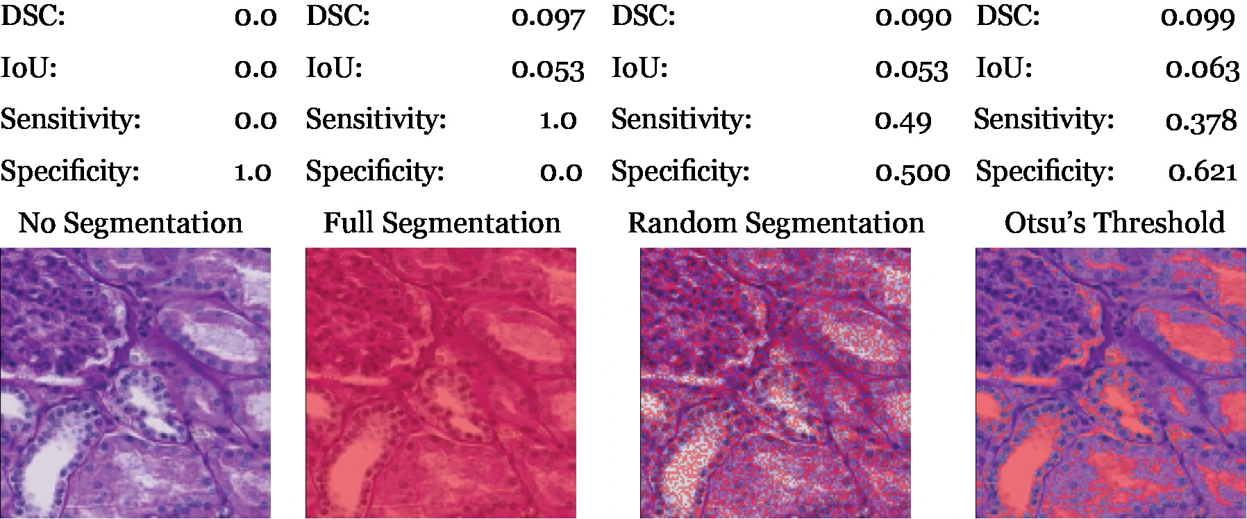
Table 1. Comparison of different algorithms. The metrics are calculated by averaging across the entire training set. The full and no segmentation scores demonstrate the class proportions.
U-Net

Figure 2. The U-Net architecture, a down-sampling encoder extracts information into many feature channels which are then up-sampled to return to the original resolution. Arrows represent operations, blue boxes are multi-channel feature maps and white boxes are copied feature maps.
U-Net is a fully convolutional neural network which was introduced by Ronneberger et al. where it was successful in segmenting neuronal tissue in electron microscope data. U-Net is widely used in medical image segmentation. U-Net's architecture is shown in figure 2, it contains no fully connected layers so can accept any resolution image as input.
For the following experiments a standard 90-10 random train-test split was used. U-Net's logits were passed through a softmax to normalize results into a probability distribution.
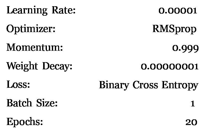
Table 2. Settings and hyper-parameters initially used to train the U-Net the optimizer and batch size match the original U-Net paper.
Normalization and Image Transformation
The model is initially trained without normalizing the tiles. Figure 3 compares DSC during training for normalized and raw tiles. The tiles are normalized with Albumentations with a mean and standard deviation pre-calculated from the entire training set (this technically is data leaking between training and validation sets).
Applying normalization allowed the epoch loss to decrease more quickly, this could be due to overfitting, but the validation shows an
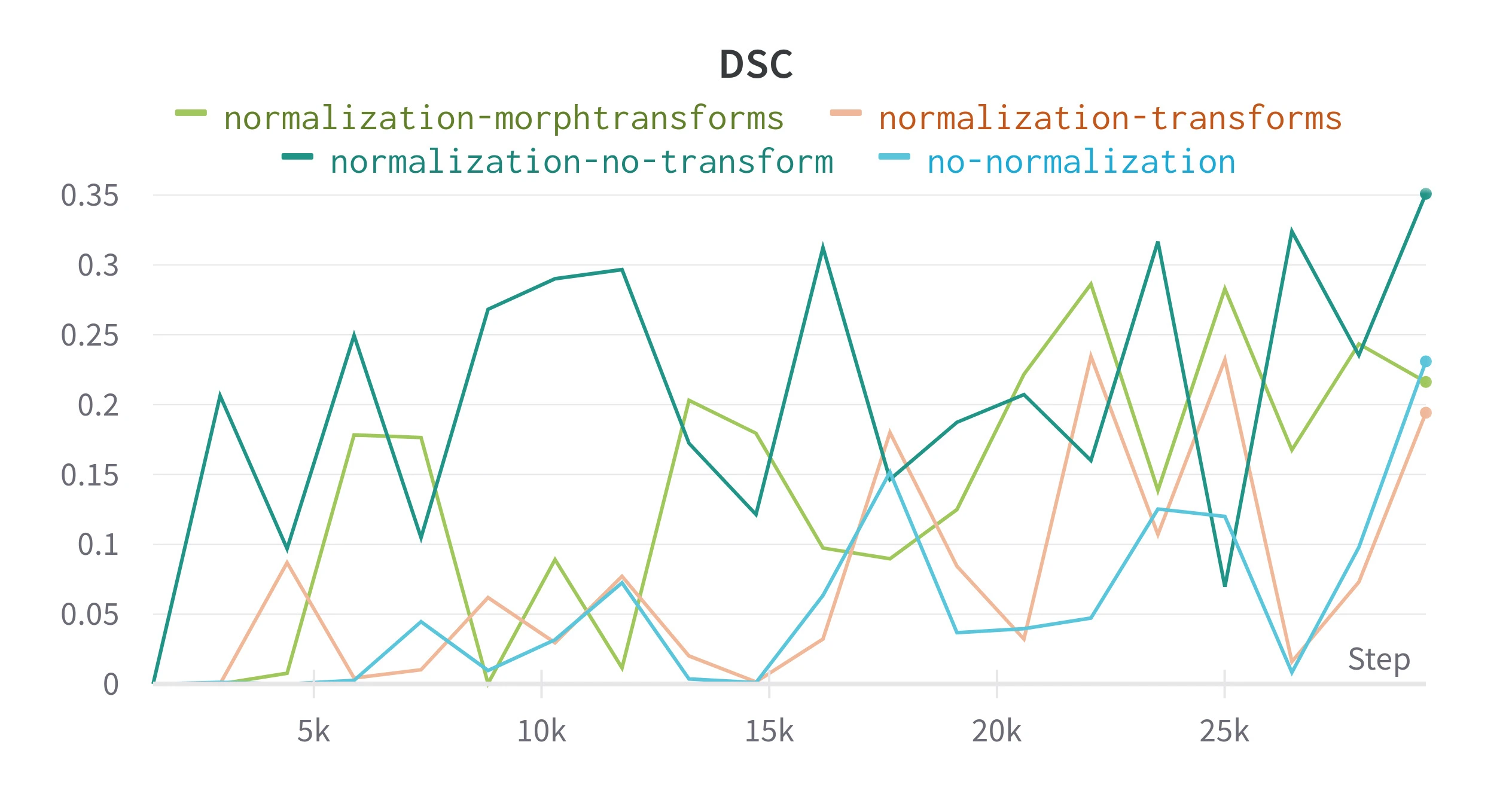
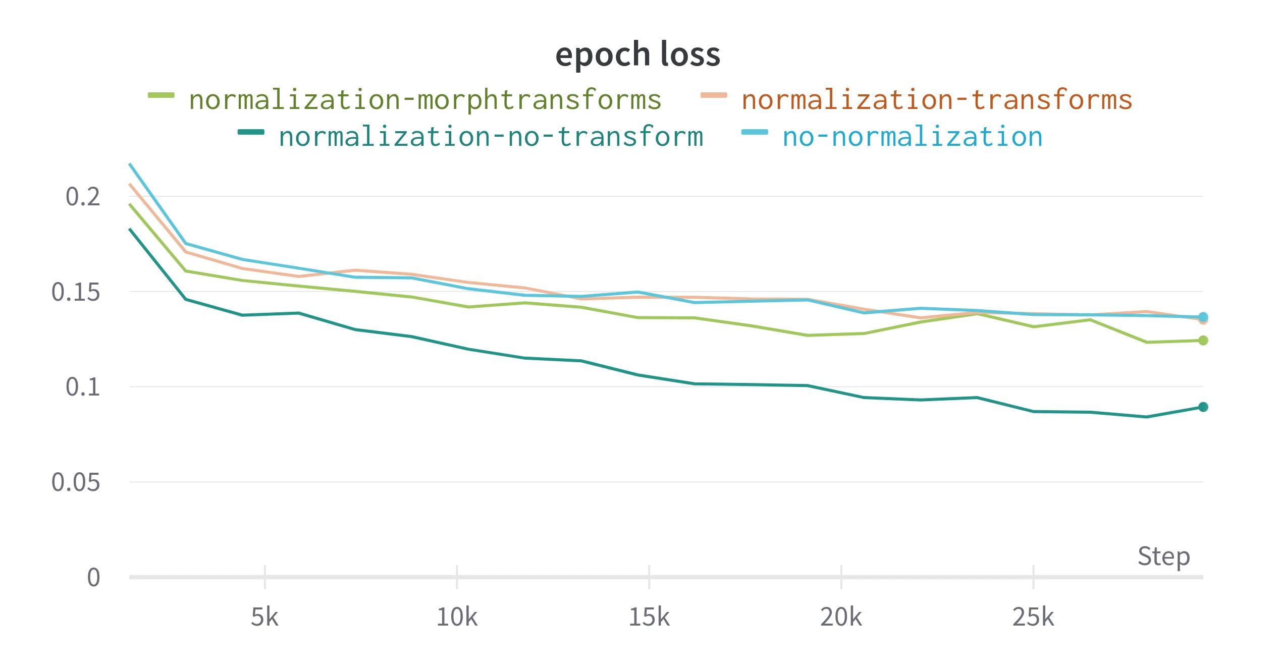
Figure 3. Result from training with different image pre-processing techniques. Epoch loss is the average loss for each training epoch, all other metrics are recalculated on the validation split at the end of an epoch. transform applies random morphological and color transforms using Albumentations, morphtransform only applies the morphological transforms.
Batch Size
The U-Net paper suggests a batch size of
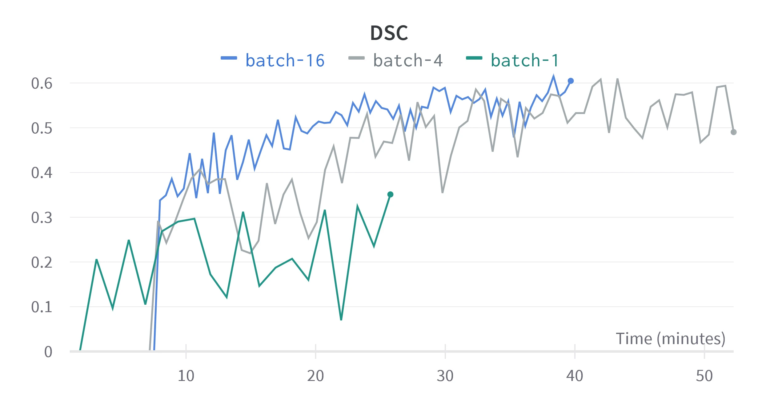
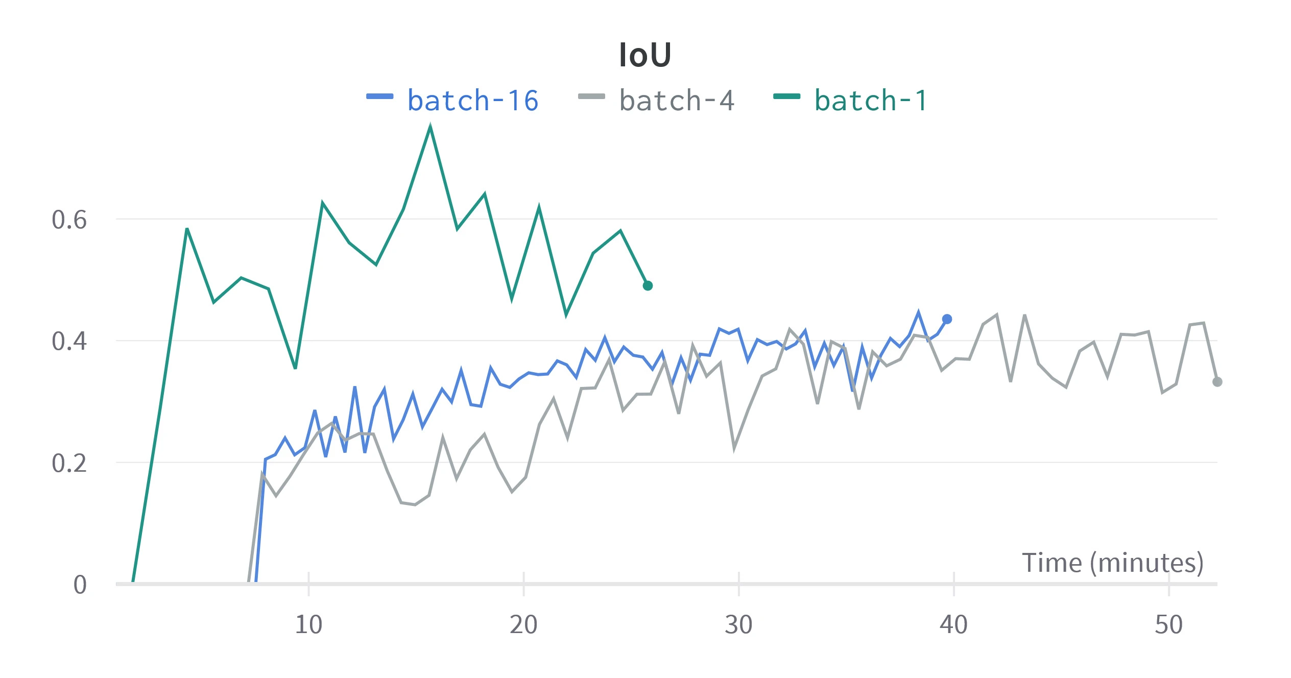
Figure 4. Validation metrics for different batch sizes. The horizontal scale is relative time since training started, since we are concerned with performance over equivalent training time.
Figure 4 shows that as batch size increases, IoU and DSC take longer to improve but show less variance, as predicted by Kandel et al. Higher batch sizes seem to reach a greater peak DSC, but IoU shows a greater peak for low batch sizes, this may be because more epochs are required to converge. A batch size of
Loss Function
The loss function measures how far a predicted label is from the ground truth. Binary Cross Entropy (BCEwithLogitLoss) is a widely employed loss function in semantic segmentation because of its stability. There exist other common semantic segmentation loss functions, which include focal loss, and combo loss. With the help of bigironsphere's Kaggle notebook the loss functions which are not built-in can be implemented in PyTorch. See Jadon et al. for the mathematical definition of these loss functions, my focal implementation sets
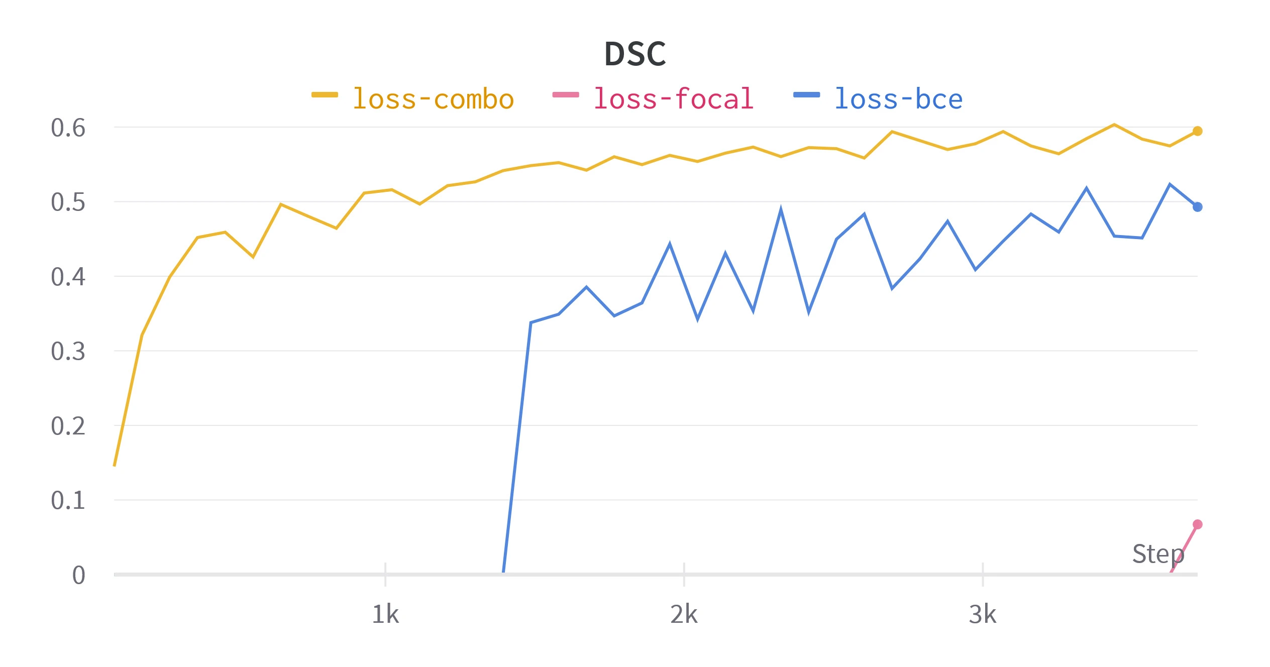

Figure 5. Validation metrics for different loss functions. All runs are performed with batch sizes of
Figure 5 compares these metrics over equivalent training setups. Combo loss consistently out performed BCE and focal loss, showing less variability and an
Results
After tuning these hyper-parameters a final model was trained over

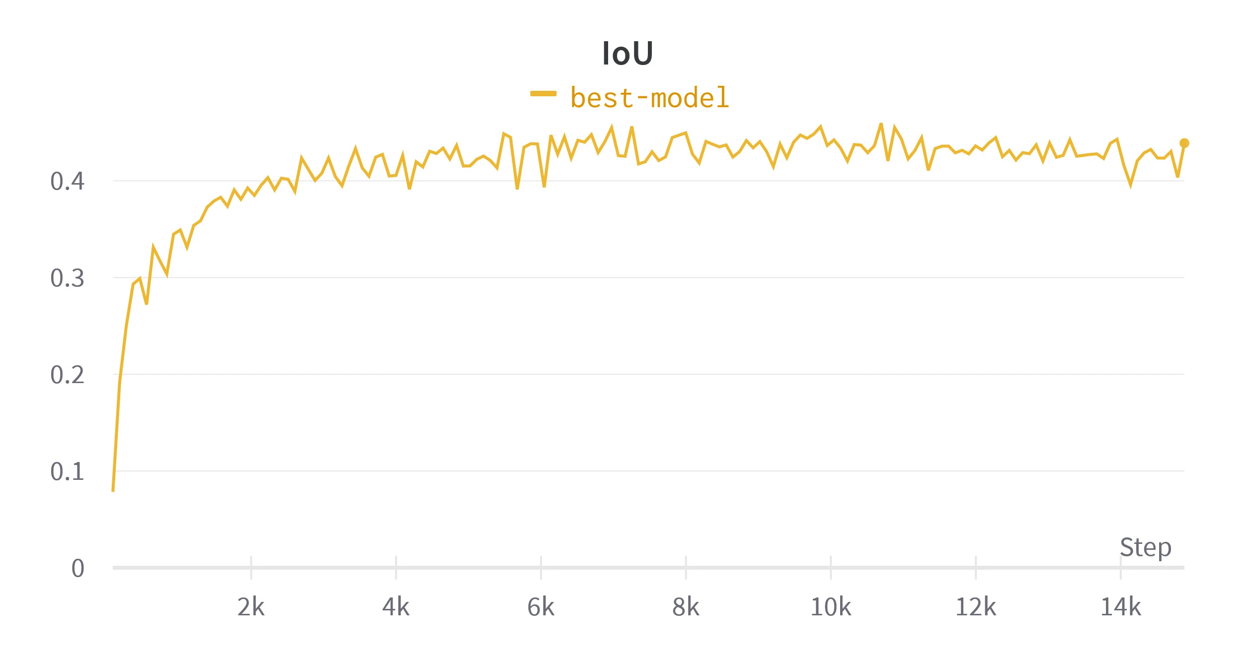

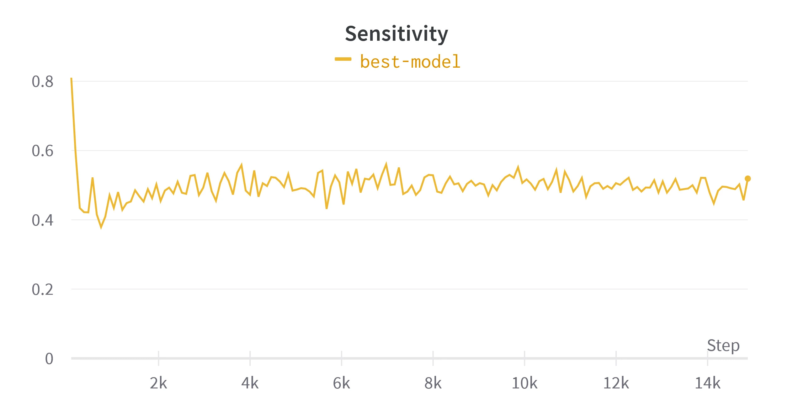
Figure 6. Validation metrics calculated while training the final model. Loss is shown per batch, rather than per epoch.

Table 3. Metrics over validation set from the models at 40th, 80th and 160th epoch with an example. Refer to table 1 for examples of these metrics on simpler segmentations.*
Conclusion
This article examined different techniques and parameters when applying semantic segmentation techniques to the HuBMAP - Hacking the Human Vasculature competition. We found that normalization of input images allowed the loss to decrease more quickly. Applying random morphological or color transformation did not seem effective on this data-set. For the standard U-Net architecture, Combo loss outperformed the simpler binary cross entropy loss and focal loss. Greater batch sizes decreased loss variance at the cost of training time and should be tuned for each data-set.